A Gentle Introduction to Modern Portfolio Theory (MPT)
A Mathematical take on: "Don't Put All Your Eggs in One Basket"

You probably heard your grandma saying:
Don't put all your eggs in one basket.
It sounded like good advice, but will you base your investment strategy on a saying? Why split bets on apples and oranges if clearly apple stock prices are skyrocketing?
The key is thinking in terms of both risks and returns. It's easy to focus solely on returns.
I look at a stock's price, notice it's up by 10% from last year, and think, "Cool, I made 10%!" But then, what about the risk?
The missing piece is certainty—how sure are you that this stock will continue growing 10% annually? Over five years?
This level of certainty, or rather the lack thereof, is what we call risk.
In this post, Modern Portfolio Theory is broken down with a simple formula for analyzing risk and returns, demonstrating mathematically why diversification can lower investment risk. Understanding this helps make smarter financial choices and build stronger plans for your money and life decisions generally.
Let's define Risk and Return
You have $1,000: $500 buys one stock (Asset A) and $500 buys another (Asset B).
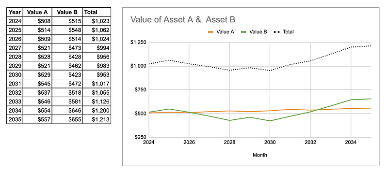
After 5 years:
The $500 in Asset A became $521 in 2029, while the $500 in Asset B became $463.
After 10 years:
The $500 in Asset A became $554 in 2034, while the $500 in Asset B became $646.
Asset A outperformed short-term (5 years), but Asset B exceeded it long-term (10 years).
How do we quantify how profitable one asset is?
Return is calculated via:
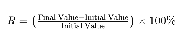
Asset A's return after 5 years: R = (521 − 500) / 500 = 4.2%; after 10 years: 10.8%.
Asset B: −7.4% (negative, indicating losses short-term), but after 10 years: 29.2%.
However, Asset A's value never fell below its original amount, unlike Asset B, which sometimes dropped below the initial $500. Asset A is less risky; Asset B is riskier.
How do we quantify how risky one asset is?
Plotting yearly returns (subtracting prior year's value, dividing by prior year's value):
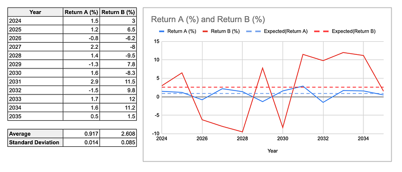
Dotted lines represent average yearly returns, or the Expected Value—fancy statistician language!
Asset B's Expected Value (2.6%) exceeds Asset A's (0.9%), as expected from B's stronger 10-year growth.
However, Asset B fluctuates more than Asset A. The blue line remains stable; the red line swings significantly. These swings represent what we call risk. Variance or Standard Deviation measure this volatility. The data confirms: Asset B's standard deviation (0.085) exceeds Asset A's (0.014).
In an ideal world, we would love assets with high returns and low risk.
How do we combine assets to reduce their overall risk?
Python demonstrates this:
import numpy as np

stock_1 = np.random.normal(loc=0.10, scale=0.5, size=10000)
stock_2 = np.random.normal(loc=0.10, scale=0.5, size=10000)
Two assets monitored over 10,000 years with Expected Value of 10% and Standard Deviation of 50%.
Combining both in one portfolio with equal weights:
def stats(*stock1):
    portfolio = np.array(stock1).sum(axis=0) / len(stock1)
    print(f"Expected Value: {portfolio.mean():.1%}, Standard Deviation: {portfolio.std():.1%}")

stats(stock_1, stock_2)

# Result:
# Expected Value: 10%, Standard Deviation: 35%
The portfolio's Expected Value matches individual assets (10%). But the portfolio's Standard Deviation is 35%, compared to 50% individually.
Magic! With 100 stocks:
stats(*[
    np.random.normal(loc=0.10, scale=0.5, size=10000)
    for _ in range(100)
])

# Result:
# Expected Value: 10%, Standard Deviation: 5%
Multiple assets maintained return while significantly reducing risk.
Don't skip the math, trust me
Two reasons require understanding the mathematics:
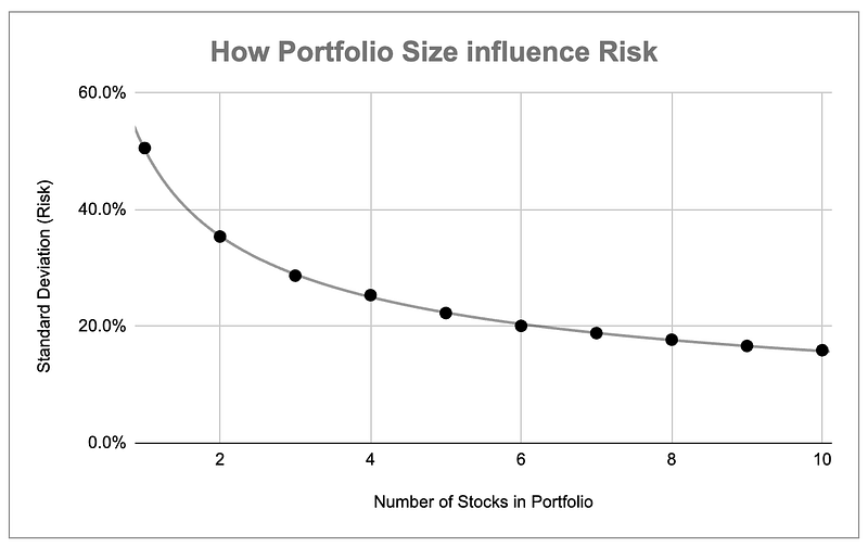
- Estimate risk reduction from diversification
- Know when this magic stops working
The first is straightforward—run simulations across multiple portfolio sizes, plot results, and derive the relationship between stock count and risk.
The second reason matters most. The formula for portfolio standard deviation:
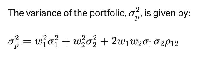
Weights are w₁ and w₂, individual standard deviations are σ₁ and σ₂, and ρ₁₂ is the correlation coefficient between asset returns.
Assuming equal 50% weights and identical standard deviation (σ):
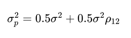
Pay special attention to the correlation coefficient (ρ₁₂).
When perfectly correlated, ρ₁₂ = 1. When inverse, ρ₁₂ = −1. When uncorrelated, ρ₁₂ = 0.
Effect on portfolio standard deviation:

In the example, assets were uncorrelated (ρ₁₂ = 0), yielding portfolio standard deviation of 35% from two 50% standard deviation assets.
But how about positively or negatively correlated assets?
Best case: negatively correlated assets (ρ₁₂ = −1) approaching zero risk!
Worst case: positively correlated (ρ₁₂ = 1) yields portfolio risk matching individual assets.
Conclusion
Diversification works, and the math proves it. However, diversification only works if your portfolio is really diverse.
If you buy stocks that move together, your diversification is just a pseudo-diversification.
Tarek Amr, January 1, 2024